Every Forex trader wants to know how risky their strategy is and what is the chance to lose a part of the account or the entire balance. This chance is called the risk of ruin. Since usually Forex traders know their win/loss ratio and the average size of their winning and losing positions, calculating the risk of ruin should be relatively easy. Or should it? Unfortunately, it isn't that simple.
The risk of ruin is a known problem in probability theory and, to some extent, it can be solved using the laws and formulas of this theory. Assessing the risk of ruin in Forex is a very complex task that requires a lot of research and calculating powers in exponential dependence on the desired level of accuracy.
The most popular ways to calculate the risk of ruin of a Forex strategy are two static formulas for the fixed position size and fixed fractional position sizing employed currently by many Forex social networks (e.g., FXSTAT, Myfxbook, and others). The formulas were presented by D.R. Cox and H.D. Miller in The Theory of Stochastic Processes and are publicly available in various sources (e.g., Minimizing Your Risk of Ruin by David E. Chamness in the August 2009 issue of the Futures Magazine). They may seem very complex at a first glance, but you can actually compute them using a calculator or an Excel spreadsheet.
Risk of ruin with fixed position size
Fixed position size condition suggests that the Forex trader won't be increasing or decreasing position size with new wins or losses. For example, if one starts with $10,000 account balance and 1 standard lot per position, dropping to $1,000 balance or advancing to $50,000 balance won't change that 1 lot position volume. The probability to lose a part of balance is exponentially proportional to the standard deviation of the account and is inversely exponentially proportional to the size of this part and the average return per trade. The formula for the risk of ruin is the following:
where:
- e is the Euler's Number (~2.71828),
- A is the average return ratio per trade (e.g., if your positions returned 2% of your account on average, then A = 0.02),
- Z is the part of the account, whose risk of losing you are assessing (e.g., to calculate the risk to lose 40% of an account, Z = 0.4),
- D is the standard deviation of your trades' returns (should be calculated in a relative form, not in currency units).
Note:
Example 1:
The risk to lose 10% of the account balance, considering a 2% mean return on a position and a standard deviation of 7%:

Example 2:
The risk of complete ruin (100% of the account balance), considering a 1.5% mean return on a position and a standard deviation of 1%:
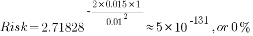
It is easy to notice that this formula calculates the risk of ruin for the infinite number of trades. According to it, the risk of loss will always be 100% for the system that currently shows negative trade expectancy and will always be close enough (but not equal) to 0 for the high enough mean return and low enough standard deviation of returns.
Advantages:
- It is a very simple method. The formula itself can be computed using a calculator. Standard deviation is trickier, but if the account balance after each trade is known it takes just several minutes to calculate it manually. A simple cycle may calculate it inside an expert advisor or some other script.
- The result is rather precise.
- It can be used to calculate the risk of loss of any fraction of the account.
Disadvantages:
- Substitutes the actual "riskiness" of the trades with the standard deviation, which isn't entirely correct.
- Assumes that the current rate of return and standard deviation won't change over time. A combination of constant rate of return and a fixed position size is almost impossible in real life.
- Assumes a fixed position size, but losing some part of the trading account may force a Forex trader to decrease the position size (most likely, it won't be possible to use 1 standard lot position size if the account is down from $10,000 to $800, for example).
- Shows the risk for the infinite number of trades — no one trades that long.
- The accuracy isn't perfect even if all assumptions are perfectly valid for a given trading strategy.
Risk of ruin with fixed fractional position sizing
Unlike the fixed position size model, fixed fractional position sizing implies that a trader is risking a fixed fraction of his account per trade (for example, 1%; the actual value doesn't really matter here), so the profit is proportional to the account size and the loss is inversely proportional to it. As with the fixed position size, the probability to lose a part of the balance is still inversely exponentially proportional to the size of this part. The dependence of the risk on the standard deviation is still positive, and on the size of the part, it is still negative, but its nature becomes more complex. The formula for the risk calculation is the following:
where:
- e is the Euler's Number (~2.71828),
- A is the average return ratio per trade (e.g., if the positions returned 14% of the account on average, then A = 0.14),
- Z is the part of the account, for which the risk of losing is being assessed (e.g., to calculate the risk to lose 25% of the account, Z = 0.25),
- D is the standard deviation of the trades' returns (should be calculated in a relative form, not in currency units),
- ln is the natural logarithm.
Below are two examples of the risk of ruin calculation using the fixed fractional position sizing model with the same conditions as for the fixed position size examples above:
Note:
Example 1:
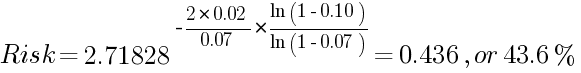
Obviously, it is only slightly lower than 44.2% of the fixed position size model.
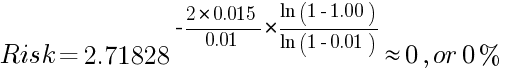
Example 2:
Since using 100% part of the account balance for the formula would imply that Z = 1, there would be an error in natural logarithm calculation (natural logarithm of 0 is not defined, but it is an infinitely large negative number). This means that it is impossible to lose the whole account if the strategy has a positive rate of returns and a fixed fractional position sizing is used:
Evidently, this formula shows a smaller risk because it assumes a fractional position sizing, which reduces the position size in case of losses, thus reducing the further losses and so on.
Advantages:
- It is still a very simple risk of ruin assessment method. Compared to the fixed position size formula, only few new steps are added, but the used data is the same.
- The result is even more precise for its model of position sizing.
- Can be used to calculate the risk of loss of any fraction of the account too.
Disadvantages:
- The same as with the fixed position size formula, the real risk is substituted with the standard deviation.
- Assumes a constant rate of return and standard deviation.
- Calculates the risk for the infinite number of trades.
Gambler's ruin problem using Markov chains
The most intuitive method to calculate risk of loss turns out to be the most difficult one in terms of the actual computations involved. The Forex risk of ruin problem can be defined as a particular case of the gambler's ruin problem, where a trader (player), starting with an initial account balance (stake), has a certain probability to win a given average profit amount and a different (or, sometimes, the same) probability to lose a given average loss amount. The trader is competing against the market (an infinitely rich adversary) — so, only the trader can get the account balance ruined; winning condition may be defined as reaching some target balance higher than the starting one.
More background research for the simple formulas of risk of loss calculation using this method can be found in the Chapter 12 of the Introduction to Probability by Charles M. Grinstead and J. Laurie Snell.
Win equals loss, same probabilities
In case when the average profit equals the average loss and the probability to lose equals the probability to win, the task of calculation the exact risk of ruin is extremely simple. The starting balance is denoted as z and the target balance is denoted as M. The risk of ruining the account before going from z to M then would be:
 / M")
Note:
Example 1:
The starting balance is $10,000 (z). There is a 50/50 probability of losing or gaining $1,000 with each trade. The target balance is $20,000 (M):
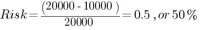
Obviously enough, the probability of going up from $10,000 to $20,000 is the same as of going down to $0 here.
Win equals loss, different probabilities
The probability to win (p) — is a chance to win (end up with profit) one position. It would be very interesting if traders could know their exact probabilities to win a particular trade, but instead the win/loss ratios are to be used here. The number of profitable trades divided by the total number of trades will be used as the probability to win. It is safe to include
The probability to lose (q) — is a chance to lose (end up with a loss) one position. For the same reasons as above, a plain win/loss ratio is the best estimate that can be used here. q = Number of losing trades / Total number of trades. Obviously, if zero profit positions were counted in the calculation of p, they aren't to be included here.
If the probability to win a particular trade isn't the same as to lose it, then a bit more complex formula should be used. The probability of winning an average profitable trade is p, the probability to lose a trade — q (p + q = 1). Then the risk of ruin is calculated as follows:
 ^ M - (q / p) ^ z) / ((q / p) ^ M - 1)")
Note:
Example 2:
The starting balance is the same — $10,000 (z), the goal is also the same — $20,000 (M), and the average win/loss is the same $1,000 per trade, but now the probability of winning is 0.55 and the probability of losing is 0.45 (a trading system with a 5% edge). To simplify calculations, it is totally safe to divide both the starting and target balances by the average win/loss to get z = 10 and M = 20. The risk of ruin before doubling the balance is calculated as follows:
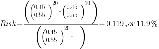
Evidently, an edge of 5% gives a Forex trader an enormous improvement in reliability of the whole trading system.
Different win/loss size, different probabilities
In reality, a Forex trading strategy rarely operates with an average profit that is equal average loss. The difference in the outcomes of winning and losing positions leads to a much greater complexity in the risk of ruin calculation. It is pointless to lay out the whole algorithm of calculation in details for this case here. Instead, it is better to provide an overview of the necessary steps, which can be easily reduced to trivial math/coding problems.
Math
The detailed information on the mathematics of the risk of ruin calculation for the general case (different win/loss size and probabilities) can be found in Kevin Brown's article The Gambler's Ruin. It is a superb work that provides an excellent explanation of this problem and the ways of solving it.
The trading process may be represented as a
In general, the formula for probability of ruining the whole account before reaching a target balance can be written as follows:
![Risk = ([q...(q)(0...0)(0)...0]M^-1Cj)/([q...(q)(0...0)(p)...p]M^-1Cj)](/img/articles/blog/2011/10/gamblers-ruin-general-case-matrix-risk-of-ruin.png "Risk = ([q...(q)(0...0)(0)...0]M^-1Cj)/([q...(q)(0...0)(p)...p]M^-1Cj)")
where:
- p is the probability of winning a trade.
- q is the probability of losing a trade.
- The upper
row-vector (a losing vector) is of the length k. The first Average loss / GCD (loss step) elements are q, the others are 0. - The lower
row-vector (a total vector) is also of the length k. The first Average loss / GCD (loss step) elements are q, the last Average profit / GCD (win step) elements are p, the rest are 0. - M-1 is the inverse matrix of the coefficient matrix M. M is a k×k matrix that has 1 in all of its main diagonal elements. In addition to 1 of the diagonal, each column may contain up to two
non-zero elements: -p — positioned below the main diagonal, with the vertical offset from it equal to the win step; -q — positioned above the main diagonal, with the vertical offset from it equal to the loss step. - Cj is the
single-column matrix (vector) of size k where all elements equal 0, except for the element at position j (starting state), which equals 1.
In the above example, the matrix M would look like this:

And if populated with values:

And the vector Cj would look like this:

While matrix/vector multiplication is trivial, inverting a matrix bigger than
Optimization
The example case is pretty simple, the matrix is only 9×9 — its inverse can be calculated pretty fast without any optimization. But what if the GCD of the strategy is $1? For example, if the average loss is $1,113 and the average profit is $1,109, the GCD is $1. With $2,500 starting balance and $5,000 target, that is a
Firstly, it is important to keep the M-1 matrix as small as possible. Optimally, k should be less than 500, if the aim is to solve this problem in reasonable time (several seconds).
Secondly, the required memory can be reduced significantly: the losing vector can be stored inside the total vector (it is known where the q's in the losing vector stop and the 0's begin), and the results of the LU decomposition can be stored inside the main matrix (M — it can be discarded after the decomposition).
Thirdly, both Ly = I and Ux = y can be solved for one column (jth), instead of the entire k×k matrix. That same column will also be a result of multiplication with Cj. This is because if the entire k×k matrix is calculated and then multiplied by Cj, the result will also be just the jth column of the matrix, because of all the zeros in Cj.
Lastly, it is possible to calculate the product of the losing vector with the jth column and the product of the total vector with that column simultaneously, as the first loss step iterations will be the same during that calculation while other iterations won't be needed in case of the losing vector.
Implementation
Here is the example PHP code that uses the above algorithm to find the risk of ruin for the earlier example:
/*
  Starting balance:      $2,500.00
  Target balance:        $5,000.00
  Avg. losing trade:     $1,500.00
  Avg. profitable trade: $1,000.00
  Loss probability:      30%
  Win probability:       70%
*/

// Greatest common divisor = $500.
$begin_state = 5; // Starting balance divided by GCD.
$N = 9; // The number of transitional states; k in the article.
$loss_step = 3; // Loss size divide by GCD.
$win_step = 2; // Win size divide by GCD.
$q = 0.3; // Loss probability.
$p = 0.7; // Win probability.

// Filling the Cj vector.
for ($i = 0; $i < $N; $i++)
        if ($i == $begin_state - 1) $unitary_vector[$i] = 1;
        else $unitary_vector[$i] = 0;

// Filling the loss vector and total vector. The loss vector is actually a part of the total vector.
for ($i = 0; $i < $N; $i++)
        if (($i - $loss_step) < 0) $total_vector[$i] = $q;
        else if (($i + $win_step) >= $N) $total_vector[$i] = $p;
        else $total_vector[$i] = 0;

// Filling the main matrix.
for ($i = 0; $i < $N; $i++)
        for ($j = 0; $j < $N; $j++)
                // The main diagonal is always 1.
                if ($i == $j) $a[$i][$j] = 1;
                // The elements above the main diagonal are about losing.
                else if ($j == $i + $loss_step) $a[$i][$j] = -$q;
                // The elements below the main diagonal are about winning.
                else if ($j == $i - $win_step) $a[$i][$j] = -$p;
                else $a[$i][$j] = 0;

// The LU Decomposition.
for ($i = 0; $i < $N; $i++)
{
        for ($j = $i; $j < min($N, $i + $loss_step); $j++) // U
                for ($k = 0; $k <= $i - 1; $k++)
                        $a[$i][$j] -= $a[$i][$k] * $a[$k][$j];

        for ($j = $i + 1; $j <= min($i + $win_step, $N - 1); $j++) // L
        {
                for ($k = 0; $k <= $i - 1; $k++)
                        $a[$j][$i] -= $a[$j][$k] * $a[$k][$i];
                $a[$j][$i] /= $a[$i][$i];
        }
}

// Solving Ly = I for one column (unitary_vector) that is equal to Cj of the Gambler's Ruin formula.
// The resulting y will also be stored in unitary_vector.
// Start from begin_state because all X's before 1 in the unitary_vector will always be 0.
for ($i = $begin_state; $i < $N; $i++)
{
        $sum = 0;
        for ($j = 0; $j <= $i - 1; $j++)
                $sum -= $a[$i][$j] * $unitary_vector[$j];

        $unitary_vector[$i] = $unitary_vector[$i] + $sum;
}

// Solving Ux = y for one column that was calculated in Ly = I.
// The resulting x will be stored in unitary_vector.
for ($i = $N - 1; $i >= 0; $i--)
{
        $sum = 0;
        for ($j = $N - 1; $j > $i; $j--)
                $sum -= $a[$i][$j] * $unitary_vector[$j];

        $unitary_vector[$i] = ($unitary_vector[$i] + $sum) / $a[$i][$i];
}

// Multiplying total_vector and its losing part by the resulting unitary_vector.
$loss = 0;
$total = 0;
for ($i = 0; $i < $N; $i++)
{
        $product = $total_vector[$i] * $unitary_vector[$i];
        if (($i - $loss_step) < 0) $loss += $product;
        $total += $product;
}
$probability = $loss / $total;
echo "Loss: $loss <br>";
echo "Total: $total <br>";
echo "Probability: $probability <br>";
The output would be:
Loss: 0.25755603952
Total: 1
Probability: 0.25755603952
So, the risk to ruin the entire account before doubling it is about 25.8% for this example.
But what if k is getting too big? In this case, mathematical rounding should be applied to the loss step, win step, and both starting and target balances, virtually truncating some of the last digits. Additionally, the target balance can be reduced. The first method influences the accuracy, but its effect becomes less important as the difference between the average loss and the average profit gets bigger.
Advantages
- If an assumption is made that the input data (the probabilities and the win/loss size) is 100% accurate, then this method offers a perfectly precise result.
- Doesn't depend on the position sizing method, but rather on the resulting average loss/profit in absolute numbers — the statistics readily available in all Forex strategy reports.
- Other input parameters are also very simple — there is no need to calculate the standard deviation.
- Simple cases can be calculated manually.
- The calculated risk is "to lose everything before reaching the target balance" — something that is achievable in contrast to the "infinite number of trades" of the previous methods.
Disadvantages
- Assumes that the main parameters of the trading strategy (the win/loss sizes and rates) don't change. That is almost never true in the real world.
- It is a very complex method.
- In many cases, requires either a lot of calculating power or a lot of rounding, reducing the result's accuracy.
Risk of ruin with Monte Carlo simulation
Monte Carlo simulation (also known as Monte Carlo method) is a model that predicts the probability of different outcomes that involve random variables. Invented by mathematician Stanislaw Ulam, it is named after Monte Carlo, a popular gambling destination in Monaco. The name seems appropriate as gambling is usually associated with chance and random outcomes.
The basic gist of the Monte Carlo method is to simulate the outcome many times with random variables getting new values on each simulation. To better understand how the method works, let us look at a hypothetical situation.
Using historical data and backtesting, you calculated the chance of loss or gain for an average trade with your trading strategy as well as the average size of your gains and losses. How to calculate the risk of ruin using this data? You can try to simulate an outcome by randomizing each trade and seeing whether your account balance will be wiped out by the end. But one simulation is of little use as it shows just one outcome among many possibilities and does not tell you likely it is.
But what if you simulate the outcome a hundred times? Thousand? Ten thousand? The Monte Carlo method suggests that by randomizing the result of each trade (a gain or a loss and, possibly, the size of the gain or loss) you gain valuable statistical data when re-running such simulations. And the more simulations you perform, the more dependable the data will be. In case of Forex trading, looking at how many times using your strategy resulted in a total wipeout of your account balance you can determine the risk of ruin.
Example of Monte Carlo simulation in Excel spreadsheet
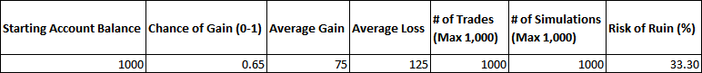
This Excel spreadsheet shows an example of a simple Monte Carlo simulation. It assumes that you know the probability of a winning trade as well as the size of the average gain and average loss.
Enter the size of your account balance in the Starting Account Balance field. Enter the chance of gain in the Chance of Gain field as a number from 0 to 1. For example, if the chance of gain is 65% then you should enter 0.65. Next, enter the Average Gain and the Average Loss in the appropriate field. If you wish to use a range instead of a fixed average number, you can easily do it by using the RANDBETWEEN function. Afterward, enter the desired number of simulated trades and the number of simulations in the # of Trades and # of Simulations fields respectively. After you filled all the fields, you can calculate the risk of ruin. To do so, go to Formulas in the main menu of Excel and click Calculate Now to the right of Calculation Options. Alternatively, you can just press
Note:
Important! The calculation can take a long time, especially on slower computers, and any click on the spreadsheet can stop the calculation, resulting in an incorrect outcome. It is better not to interact with the spreadsheet after the calculation has started until you see Ready in the bottom-left corner of the screen.
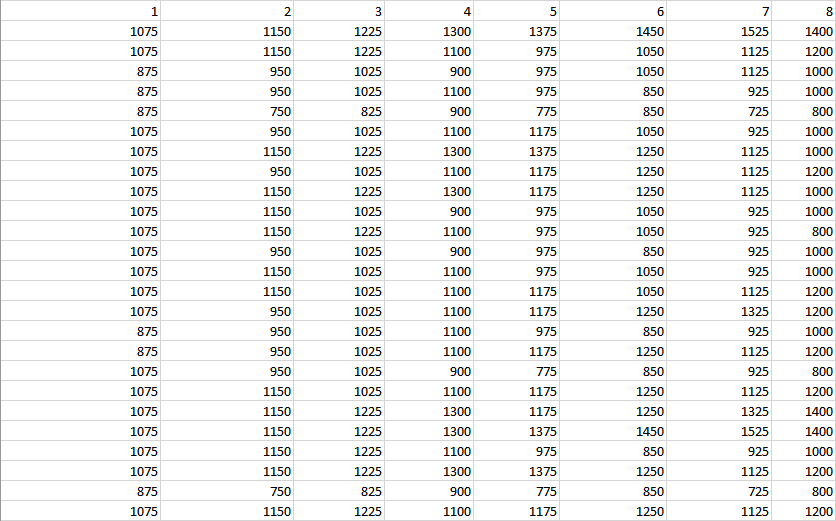
Below the table's inputs, you will see the row of trades' numbers. Below that, there are rows of the resulting account balances at each trade, with each row representing one simulation.
Each trade either adds the Average Gain amount or subtracts the Average Loss amount from the account depending on whether the random number generated for that trade is below or above the Chance of Gain value. If, at some trade, the account balance reaches zero or negative value, that simulation stops and is counted as "ruined".
If you want to have more simulations than the maximum 1,000 possible with the given spreadsheet, you can easily copy over the rows farther down — the formulas should work correctly. Same with the number of trades per simulation you can copy and paste the columns after trade #1,000 to increase the maximum number of trades.
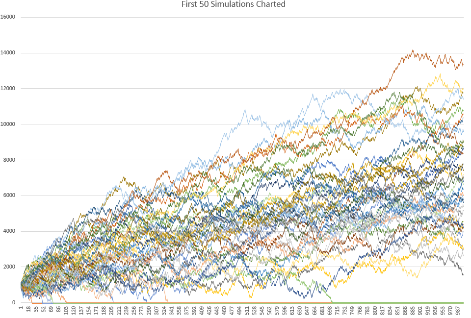
Here is the chart with an example of the first 50 simulations plotted. Note how some of them reach the zero line and remain there — those are simulations when the strategy ruined the trading account:
Advantages
- Monte Carlo simulation is a simple concept and doesn't involve complex math.
- Using multiple simulations with changing variables, you can get a more precise chance of ruin than just using simple average values.
- There are plenty of tools on the Internet for performing Monte Carlo simulations — from webpages to Excel add-ons.
Disadvantages
- Monte Carlo simulation assumes a "perfect market", meaning that it does not account for fundamental changes, be it short-term changes due to important events (like COVID-19) or long-term changes due to structural changes in how the market operates (the example of this is the "peg" and the subsequent "unpegging" of the Swiss franc to the euro by the Swiss National Bank). Such changes make the historic data used for calculations useless.
- Changing your trading strategy can also make historic data irrelevant, meaning that Monte Carlo simulation should be used only for testing consistent trading strategies.
- Monte Carlo simulation assumes that each trade is independent of the previous ones. Therefore, it is unsuitable for serially correlated strategies with trades that take into account the results of the previous trades.
Conclusion
None of the described methods is perfect. Each of them should only be used when it fits the parameters of the Forex trading strategy:
- Fixed position size formula is good when you know that the position size is fixed, can calculate the standard deviation, and the input of the losing positions into standard deviation is greater than that of the variability of the winning positions. It is a good method if you don't want to perform any complex calculations.
- Fixed fractional position sizing formula is perfect for the fractional position sizing strategies. Again, finding the standard deviation is necessary. It also needs to be formed by both the losing and the winning positions.
- Gambler’s Ruin method is recommended when you are confident that the statistical parameters of the trading system are stable (the average win/loss size, the win/loss rates) and don't mind doing some really complex calculations.
Whichever method you choose, it is important to remember that the resulting risk value shouldn't be taken too seriously on its own. Its main purpose is in comparing different strategies or the effect of the changes applied to one trading strategy. Relying on the calculated risk value as the real measure of strategy riskiness can lead to unexpected but horrible consequences.
Note: it is possible to calculate the first three types of risk of ruin by using the Forex Report Analysis Tool. Perhaps, the only free online tool that offers such functionality.
If you have any questions or commentaries regarding the assessment of the risk of ruin in Forex trading, please feel free to discuss them on our forum.